

We’re Being Deluged By Data
According to market intelligence company IDC, the “Global Datasphere” in 2018 reached 18 zettabytes. (Yes, that zettabytes!) And the problem is only going to get worse – the amount of data being generated increases relentlessly.
The data being collected by organizations can, however, give a misleading or fragmented view of the real world. A person, for example, could appear multiple times (or have multiple digital entities) within the same database, due to typos, name changes, aggregation of different systems and so on. If we try to merge two databases, how do we match entities, when the ID systems might be different or contain errors?
Entity resolution (ER) helps get to the truth. Entity resolution, which is the disambiguation of real-world entities in a database, is an essential data quality tool for, for example, businesses wanting to see the full customer journey, and to make the right recommendations, or for law enforcement trying to uncover criminal activity and the perpetrators.
Graph Databases Can Help You Disambiguate
The key of entity resolution task is to draw linkage between the digital entities referring to the same real-world entities. Graph is the most intuitive, and as we will also show later, the most efficient data structure used for connecting dots. Using graph, each digital entity or the entity attribute can be represented as a vertex, and the entity-has-attribute relationships can be represented as edges. In such an entity-attribute graph, when multiple entities share the same attributes, they will be linked together by the graph (see figure 1). By representing the entity-attribute relationship as a graph, a variety of graph algorithms (e.g. cosine similarity, Jaccard similarity, shortest path, connected component, label propagation, Louvain) can be performed for the task of entity resolution.
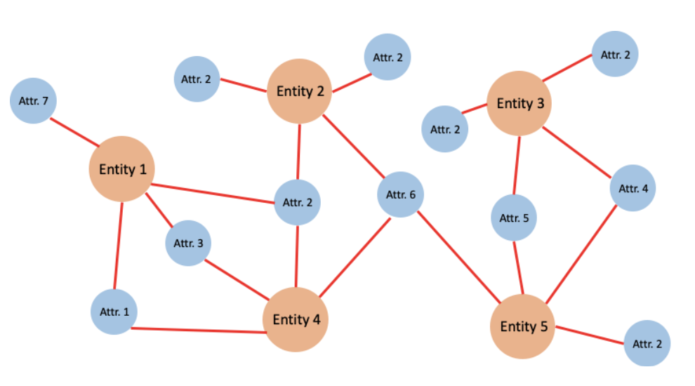
Figure 1. Each vertex in the graph represents either an entity or an attribute. The edges represent the entity-has-attribute relationship. The graph linked different entities together when they share common attributes. For example, Entity 3 and Entity 5 are linked by Attr. 4 and 5.
Solving the entity resolution problem with graph can break down into two steps, namely linking and grouping. In the linking stage, graph algorithms, such as cosine similarity, Jaccard similarity, and shortest path, can be applied for pairwise matching. Once two entities are matched, an edge can be drawn between them to represent the same-as relationship. The same-as relationship can be deterministic as well as probabilistic. In the case of probabilistic relation, an weighted edge can be used to represent the likelihood of one entity being the same as the other entity. In the grouping stage, the inserted same-as edges can greatly accelerate the computation in which graph community detection algorithms, such as connected component, label propagation, and Louvain, can be used to group the the digital entities by their real-world entities.
Graph provides an efficient approach for the entity resolution problem. A native graph database with massive parallel computing capability is the best tool to implement the approach. Solving entity resolution problems by running queries in the database not only saves the time for exporting the data to the other computing platform, but also addresses the challenge of ever-growing data size and data update. Additionally, because of the transitivity of the same-as relationship (i.e. if entity A is the same as entity B, and entity B is the same as entity C, then entity A is also the same as entity C), entity resolution requires multiple-hop queries. Such queries require multiple join operations which are computationally expensive for relational database. A graph database, on the other hand, is the ideal solution for the big data entity resolution task. In the next section, we will show how to implement a TigerGraph solution for entity resolution.
TigerGraph is Especially Adept at Uncovering the Truth
Let’s examine a real-world example of how TigerGraph disambiguates the passengers through booking records of flight tickets. Each booking record can include the ticket number, passenger first/last name, email address, phone number, departure, destination as well as other related information. An airline company can have millions of ticket records in the database. One passenger may use different email addresses, phone numbers, or names to book flight tickets. In this scenario, each booking record is a digital entity with multiple attributes. The entity resolution task is to link the tickets to the real-world entity, passenger. Without losing the generality, in this simplified example, we assume each record contains the ticket number, passenger name, email, and phone number (see table 1). The five tickets in this toy example were actually booked by the same person. Now let’s build a graph in TigerGraph to find this person.
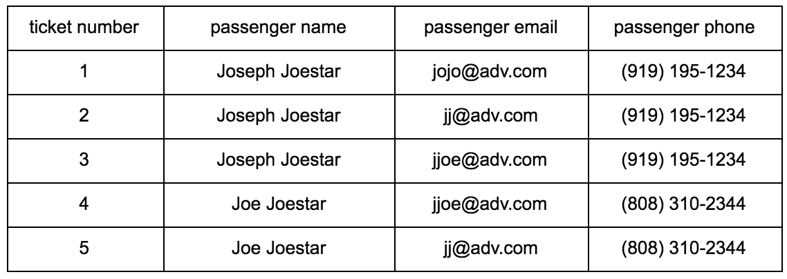
Table 1
Defining Graph Schema
We need five types of vertices in this graph. The first type of vertices is for the flight ticket (i.e. digital entity), and they can be created using the ticket number. Similarly, each of the three attributes, passenger name, email and phone, can also be represented by a type of vertice. The last type of vertex is the passenger, the real-world entity. The grouping of the digital entities will be done by connecting all the matching ticket vertices to the same passenger vertices. For the edges, we have “has” edges between tickets and the attributes, “book” edges between passengers and flight tickets, “same as” edge between passengers.
Loading Data
With the graph schema above, the data can be loaded to create the entity-attribute graph. For each record, we will use the ticket number as well as the attributes to create vertices, and connect the ticket vertex with its attribute vertices. Figure 2 shows the graph created by the sample data in table 1.
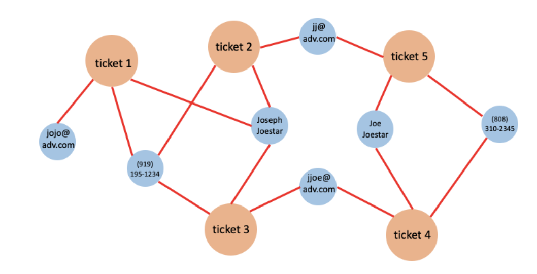
Figure 2. The graph created by loading the data in table 1.
Running Queries
The task of entity resolution can be split into three queries, initialization, linking and grouping.
1. Initialization:
In the initialization query, we will first assume each ticket was booked by a different passenger and the passenger has all the attributes (i.e. names, phones, emails) connected to the ticket. This is done by creating a passenger vertex for each ticket vertex, then inserting a “book” edge from the passenger vertex to ticket vertex as well as “has” edges to the attributes of the flight ticket (see figure 3). This step is important for the data lineage purpose. As we will see in the third step we will merge/remove the duplicated passengers, the initialization step allows us to keep the original relations between tickets and attributes.
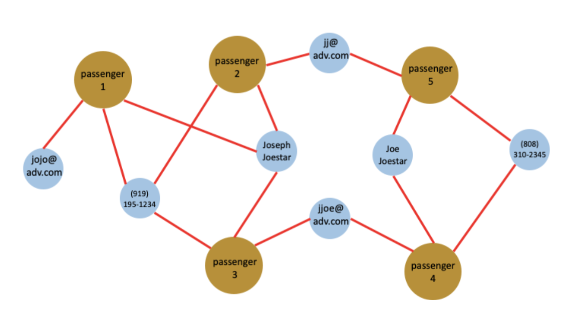
Figure 3. The initialization query assumes each ticket is bought by a different passenger and let the ticket-buyer inherit all the attributes of its ticket. For simplicity purposes, this figure only shows the passenger-attribute relations and does not show the ticket vertices in the graph.
2. Linking
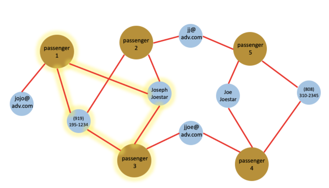
The linking query connects the entities that satisfy the matching condition. In this example, let’s assume two flight tickets were booked by the same person when they share at least two attributes. For example, ticket 1 and 3 were booked both using the same phone and name, thus we consider they were booked by the same person (see figure 3). In this case, the linking query traverses all the passenger – attribute – passenger paths and aggregates the count of paths for each pair of passengers. Lastly, the query will insert an edge between two passenger vertices if they are linked by at least two attributes.
(a)
(b)
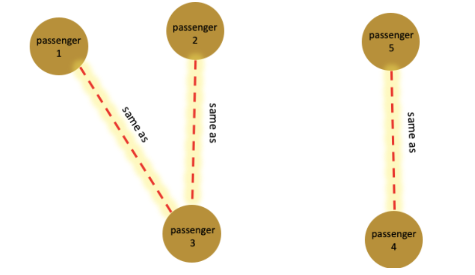
Figure 4. (a) In the above example, three same-as edges will be inserted between passenger (1, 3), (2, 3) and (4, 5) because each pair shares at least two common attributes. The connections between passenger 1 and 2 are highlighted. (b) The graph of passenger-passenger relationship after inserting the same-as edges in the linking query. For simplicity purposes, this figure does not show the ticket and attributes vertices in the graph.
3. Grouping
After the linking query finishes, all the matching passengers will be connected. The entity deduplication can be achieved by merging the connected passenger vertices together. This can be done by performing the connected component algorithm on the network formed by the passenger vertices and same-as edges. Briefly, the connected component algorithm will find the connected entities by assigning the same label to the entities in the same connected group.
The connected component algorithm can have different variation, below is one example to show the overall idea:
1. Assign a unique integer as an ID to each entity.
2. Propagate this ID to its connected neighbors, so that each vertex will receive all its neighbors’ IDs.
3. Update the old ID by using the smallest ID value received from the neighbors.
4. Repeat above steps 2 and 3 until no ID update happens.
When iteration stops, the vertices in each connected component will have the same ID. And this ID will be the smallest ID within the connected component. Above algorithm not only finds the connected entities, but also selects a “lead” entity within each connected group. The last step of the grouping query is to let the lead entities inherit all the attributes in the group and remove the other entities. The graph of passenger-attribute relations after the grouping query finishes is shown in figure 5.
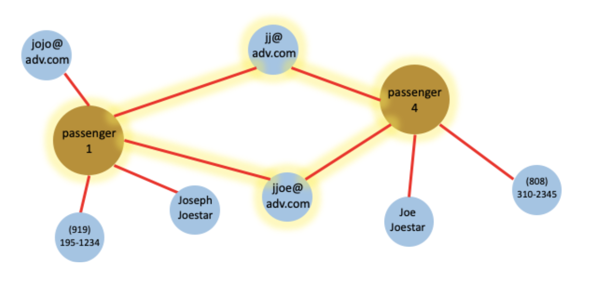
Figure 5. After the grouping query finishes, passenger 1, 2, 3 will be merged into passenger 1. Passenger 4 and 5 will be merged into passenger 4.
In some use cases, multiple iterations are needed to repeat the linking – grouping steps. For example (see figure 5) after we merge passengers 1, 2, 3 into 1, passenger 1 will have all the attributes from 2, 3 and itself. So passenger 1 can connect to other entities that it did not in the last iteration, thus new groups can be formed. Therefore, the linking and grouping shall be repeated until no more same-as edge needs to be inserted. It is also worth mentioning that in all above steps the operation on each vertex can be run in parallel, and the algorithm can fit into a map reduce framework. Above solution also works for incremental updates. When having new data or streaming data loaded into the database, we don’t need to rerun the process using all the existing data. Instead, we only need to label those newly loaded data, and process the newly loaded vertices and their neighbors.
Now Is The Time
We’ve shown that graph database is a powerful tool for entity resolution especially on a large data scale. We also examined a general approach for solving entity resolution tasks with graph algorithms has been introduced, and included a representative use case (i.e. flight ticket booking) has been discussed in detail to show how the passenger entities can be resolved by running three queries in the graph database.
Now is an ideal time for you to get started with graph databases. One of the best ways to get started with graph analytics is with TigerGraph Cloud. It’s free and you can create an account in a few minutes. Sign up here.