


How to Build an Associative Memory Capability in 1 Hour
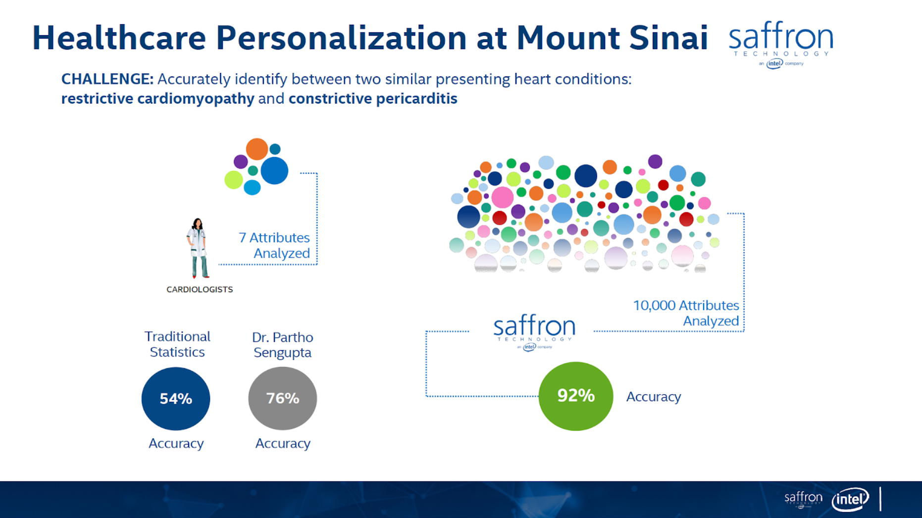
Recently I came across a wonderful presentation about Cognitive Computing and Associative Memory.
Intel Saffron is a product dedicated for predictive analytics based on the associative memory concept.
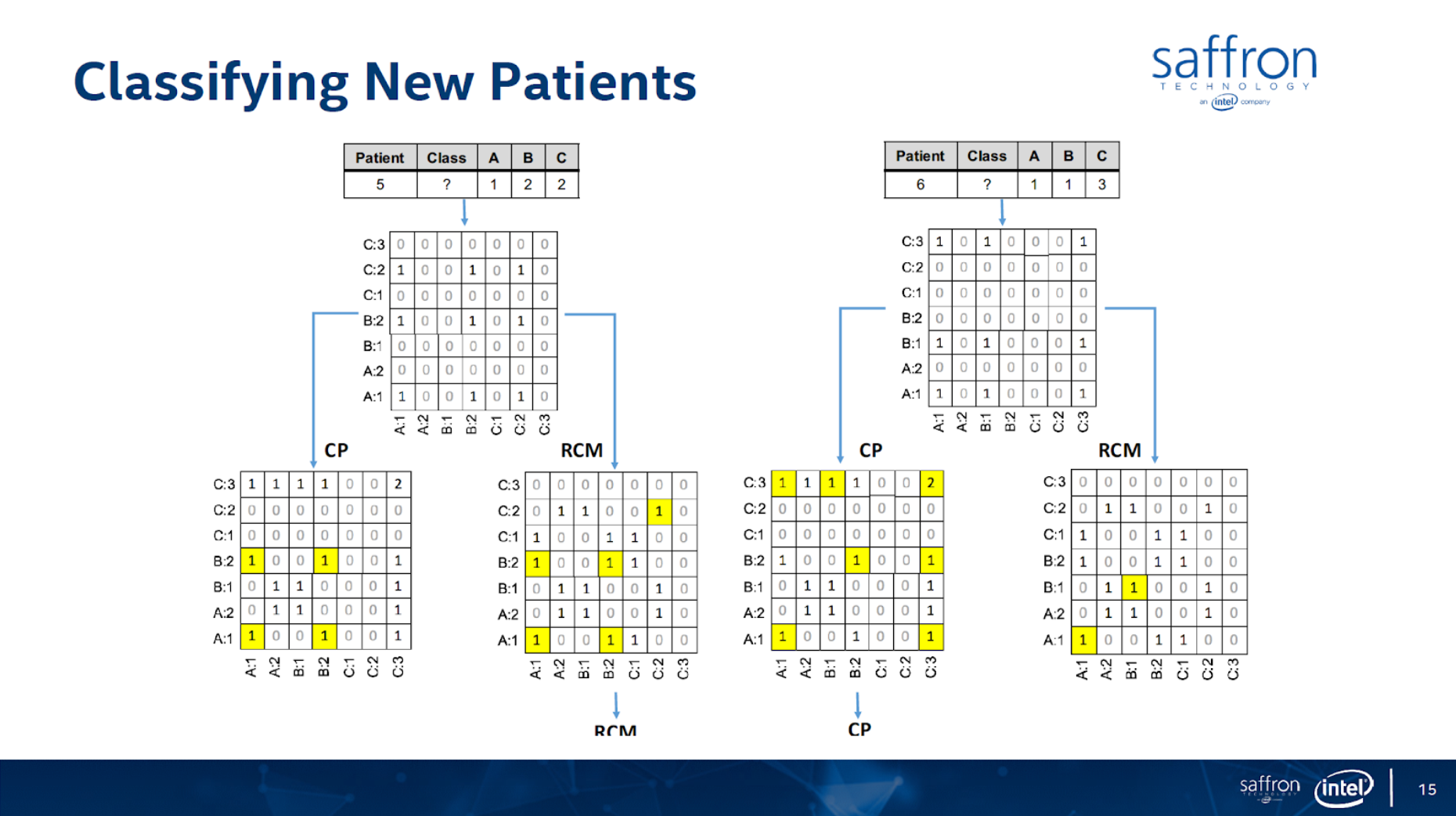
In this article I’ll show how to use graph technology for predictive analytics use cases for patient classification using the Associative Memory technology. The figures below (from https://theaisummit.com/wp-content/uploads/2016/10/Andy-Hickl.pdf) show how associative memory technology works to predict which of the two types of heart diseases each of the new patients 5 and 6 is likely to have, based on the information about patients 1, 2, 3 and 4 while patients 1 and 2 have the first type of heart disease and patients 3 and 4 have the second type of heart diseases, using matrices as associative memories.
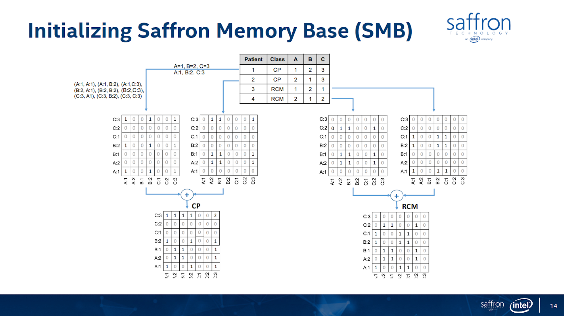
Both the concept and quality of the classification/prediction are great. The problem is that it requires lots of memory and storage for such matrices, and more importantly, it requires a lot of professional services to decide what associations to build. There are also issues of how to scale the computation/storage to a distributed architecture.
Let’s see how we can use a graph to solve this problem in 1 hour, while including all the benefits of auto-scaling, and parallel computing performance coming with a native distributed graph database. In the graph below, each patient and each dimension’s measurement is modeled as a vertex in the graph. Each disease is connected to the patients who have that disease. Each patient is connected to the vertices representing the measurements of the patient. The Graph Schema is shown below:
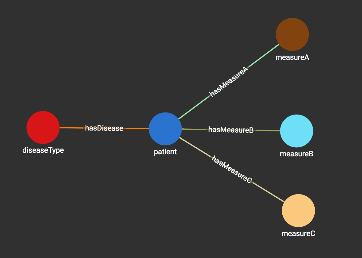
The following figure shows the data graph representing the four patients, their type of disease and their measurements.
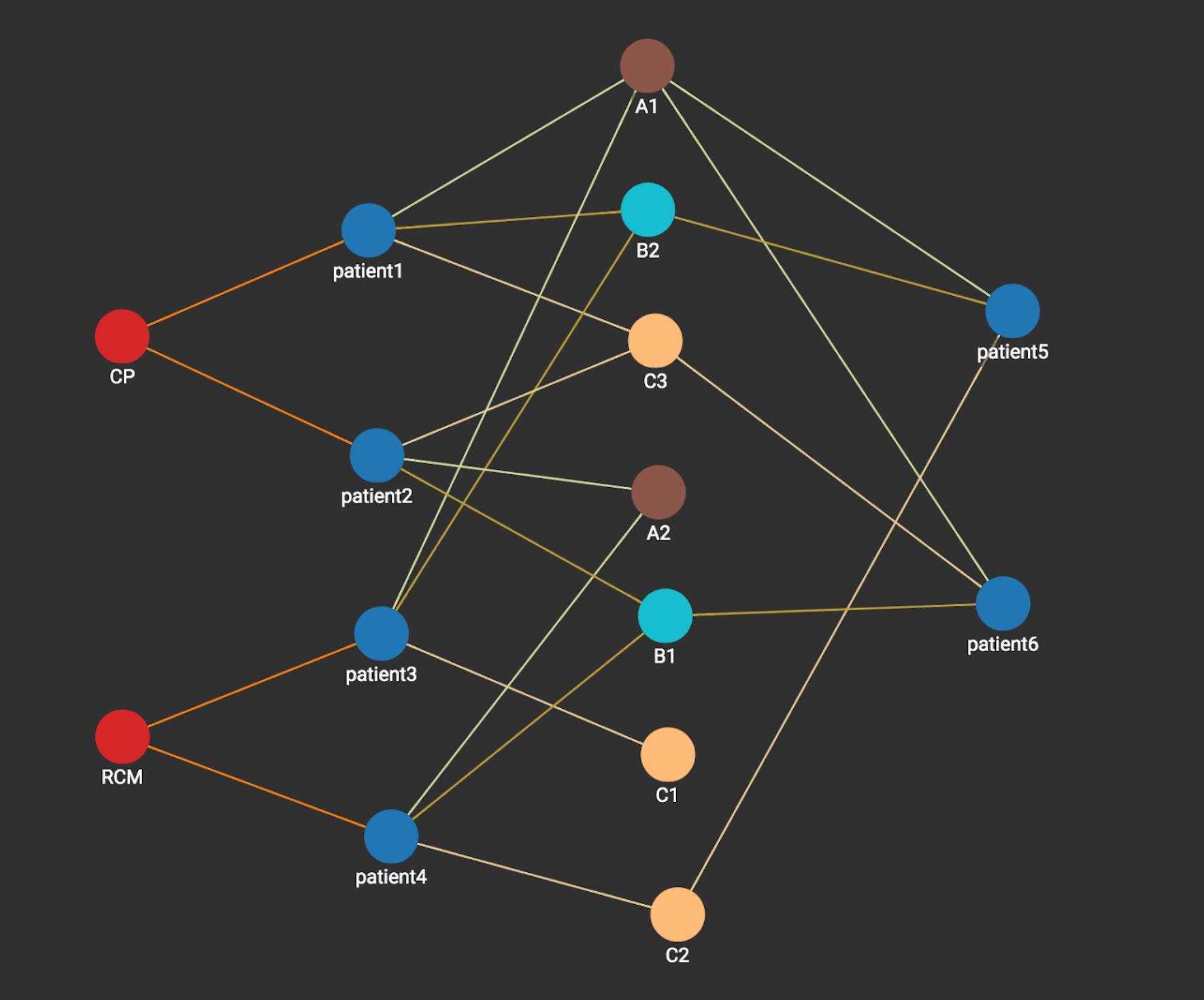
Now we need to do prediction for patients 5 and 6. Let’s pick up the prediction for patient 5 as an example. This becomes a graph problem of whether the patient is more ‘similar’ to heart disease CP or heart disease RCM via the connections through existing patients (1 to 4). With a native parallel graph technology, this problem can be solved very efficiently.
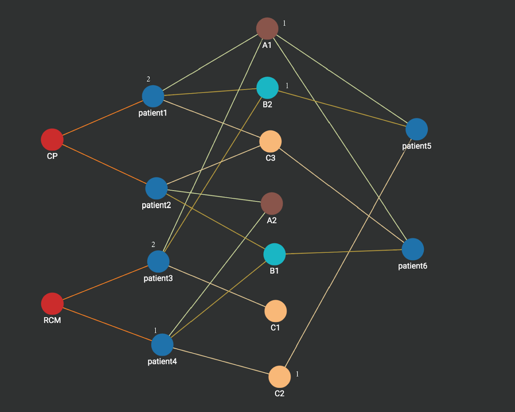
Step 1: we start from the vertex patient5, its measurement vertices A1, B2, C2 are activated and each vertex is associated with an integer count with value 1 (sometimes called an Accumulator in Native Parallel Graph).

Step 2: A1,B2,C2 activates its neighbors patient1, patient3, and patient 4. Each activated patient is associated with an integer count which stores the number of times it’s activated. Notice that patient1 and patient3 each has a count value of 2 since each is activated two values (by A1 and B2), while patient4 is activated only one time (by c2) and thus has a count value of 1.
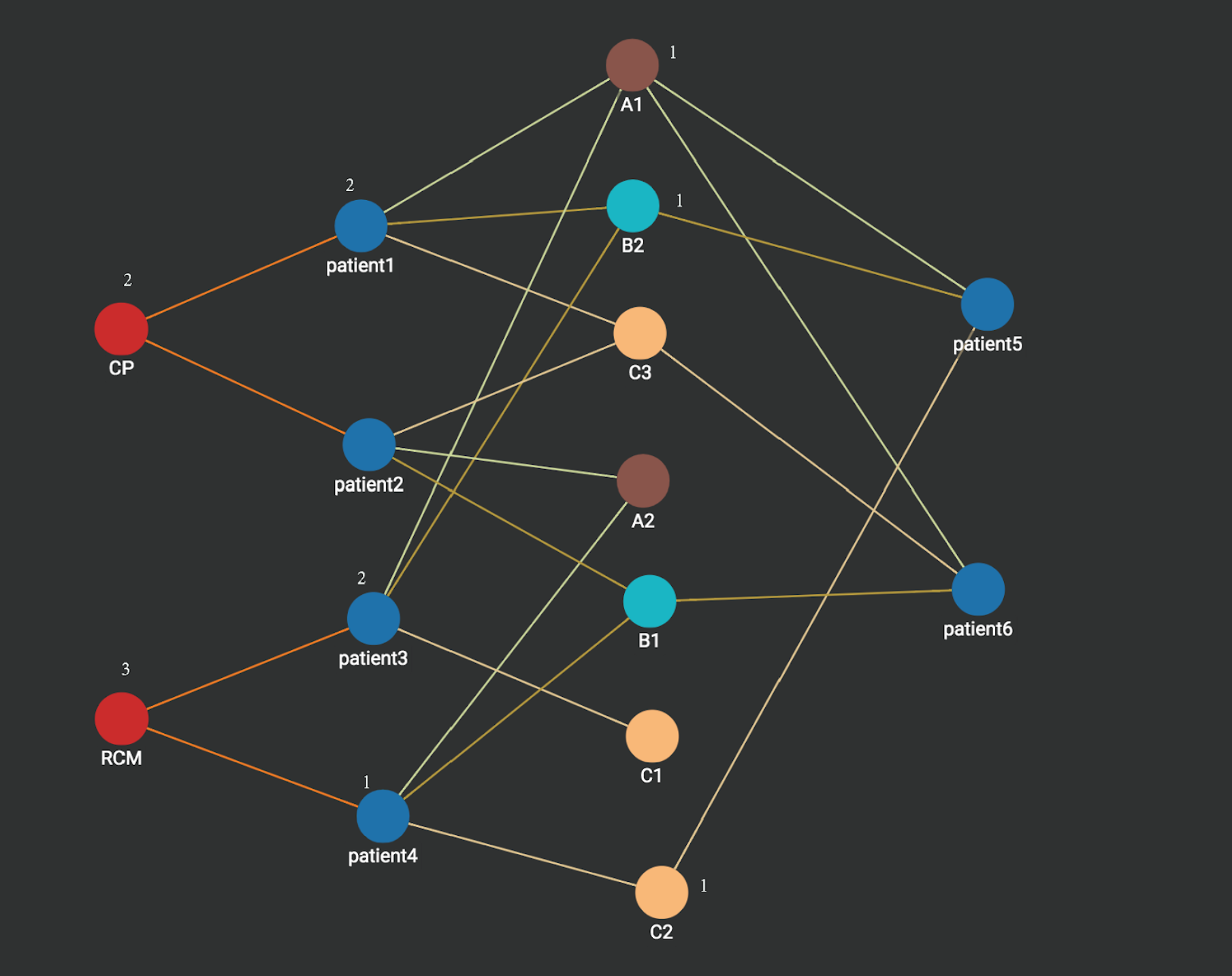
Step 3: Heart disease vertices CP and RCM are activated. Each disease vertex is associated with a count which stores the sum of the counts of its connected vertices activated in the last step. We can see heart disease RCM vertex has the value 3 which is more than what is on the heart disease CP vertex (2). Thus the prediction for patient 5 is heart disease RCM. Similarly, if we apply the same graph computation, the prediction for patient 6 is heart disease CP.
Note that more complex/weighted similarity computation can be easily modeled and used in the above type of computation in a native parallel graph which uses the property graph model. For example, we could have a trust score for each measurement for each patient. We could also assign different weights to different types of measures in computing similarity. For example, A measurements can be more important in prediction than B measurements. All this information can be easily added as either vertex attributes or edge attributes and used in run time similarity computation.