An Efficient Process for Cycle Detection on Transactional Graph

Cycle detection, or cycle finding, is the algorithmic problem of finding a cycle in a sequence of iterated function values. Cycle detection problems exist in many use cases in the banking and financial services industry. For example:

• Detecting the circular transaction patterns in AML use cases
• A group of accounts transfers money within the group to forge higher income for loan fraud
• Stock circular trading to raise the stock price

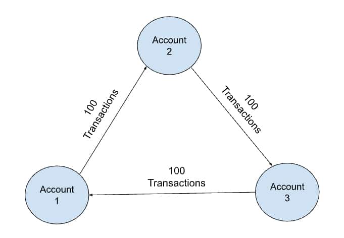
Each follows the same pattern, in that a sequence of transactions has been conducted in order of time and the sender of the first transaction is the receiver of the last transaction.

Cycle detection is a very important graph feature that indicates fraudulent behaviors or misconduct. And usually, the calculation is done on a transactional graph, where transactions can be performed between two accounts.

In this article, we will introduce a multi-step cycle detection procedure on transactional graphs that is lightweight, efficient, and able to run on very large datasets.

Challenges

When directly applying the Rocha–Thatte algorithm on the graph, we will face the challenges below:

High Complexity To Apply Restrictions

In the vast majority of real-life use cases, restrictions will be applied to the cycles such as, in each cycle, the gap between one and the following transaction should be no longer than a specific period of time. Or the following transactions should have a similar amount to the previous transaction.

For each account, the restriction check will have to be performed in O(dout*p) complexity, where “dout” is the number of outgoing transactions, and p is the number of paths going through this vertex. This means that, for every incoming path of an account, it will have to check if every outgoing transaction can be a following transaction of the candidate cycle path or not. And the number of paths going through an account is much larger than the number of incoming transactions of an account. The reason is that every incoming transaction will initiate one candidate cycle path and any upper-stream transactions of the incoming transactions can initiate a new candidate cycle path going through the downstream accounts.

High RAM Consumption

By nature, the cycle detection algorithm has very high space complexity, since it will have to propagate all the cycle candidate paths along the way to detect the cycles.

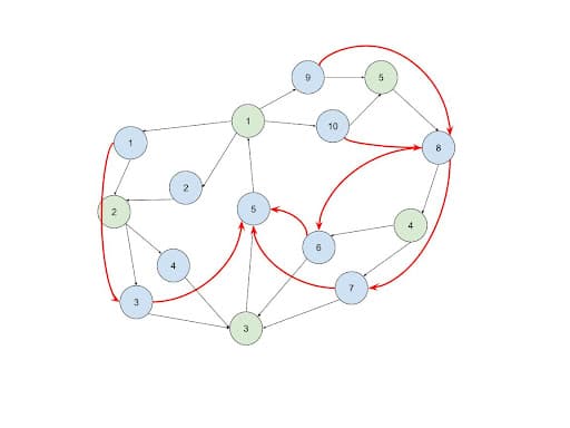
Another reason can be as one of the features of the transactional graph, the cash flow can diverge from accounts and also converge into a certain account. This means for the same account that initiated the cycles, all the possible combinations of the cycles will be detected and returned as a result. This leads to extremely large memory consumption. In the example in the image below, there can be up to one million cycles starting from Account 1.

When longer paths are present to be detected, the graph will propagate longer paths around and also tend to have more combinations.

Large Data Size

Usually, banking and financial services have transactions numbering in the billions. This results in transactional data sets ranging from 100GB to 10TB or more.

The Innovation

The innovation is to introduce a direct connection between accounts and transactions and use the Strongly Connected Component algorithm to filter out cycle path candidates to lower the RAM consumption and improve performance.

The Schema

For our example, we propose a solution and experiment using a TigerGraph implementation. TigerGraph is a massive parallel processing (MPP) graph analytical platform.

Let’s start with a simple schema:

Vertex Types

• VERTEX Account(PRIMARY_ID id STRING, scc_id UINT) 
• VERTEX Transaction(PRIMARY_ID id STRING, amount FLOAT, tran_date UINT, scc_id UINT, is_cycle_tail BOOL) 

Edge Types

• DIRECTED EDGE Account_Account(FROM Account, TO Account) WITH REVERSE_EDGE=”reverse_Account_Account”
• DIRECTED EDGE Trans_Trans(FROM Transaction, TO Transaction) WITH REVERSE_EDGE=”reverse_Trans_Trans”
• DIRECTED EDGE Send(FROM Account, TO Transaction) WITH REVERSE_EDGE=”reverse_Send”
• DIRECTED EDGE Receive(FROM Transaction, TO Account) WITH REVERSE_EDGE=”reverse_Receive”

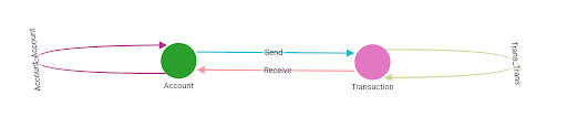
In this schema, between the Account and Transaction vertices there are two edge types, Send and Receive. The other definitions are for storing the preprocessing results; more details will come later.

A Side Note: Why Define a Transaction as a Vertex?

Yes, it is possible to define transactions as edge types. However, there are a few reasons for not doing so and defining transactions as a vertex type.

1. Algorithms like SCC are at the vertex level, so we won’t be able to find the SCC of Transactions if they are edges
2. Some of the optimizations are based on the relationship between Transactions, so defining them as vertices allows us to create direct connections between transactions (step #3) to mitigate challenge #1.

The Proposed Workflow

The proposed workflow has five steps. Each of the first four steps prepares the way for its following step. In the last step, the result is calculated. Another way to describe this is the first four steps are preprocessing steps for the final step. Let’s look at the intuition of each step and its detailed approach.

Connect the Entities

Intuition: In most of the transactional/trade graphs, the number of transactions is dominantly larger than the number of accounts by a few orders of magnitude. This way, aggregating the actions between two entities into one single edge can largely reduce the scale of step #2, which utilizes the result of step #1.

Implementation: Consolidate the transactions into directed Account_Account edges based on their directions. After executing the first step, a network of directed connections between entities will be created.

Run SCC on the Account Network

Intuition: A graph is said to be an SCC (strongly connected component) if every vertex is reachable from every other vertex. Based on the definition of SCC, all vertices on a cycle must exist in the same SCC. No cycle can cross more than one SCC. This way, during cycle detection, if we filter out the cycle candidate paths that will go across SCCs, we can reduce the computational complexity.

Implementation: Based on the connections that were calculated in step #1, run the SCC algorithm from the Graph Data Science Library. The SCC ID of each account vertex will be stored as an attribute.

Connect the Transactions

Intuition: Establishing a direct connection between transaction vertices is an essential step of this process. The reason for connecting transaction vertices is to solve challenge #1. When we connect the transactions, we want to make sure they belong to the same SCC, follow the order of time, and also fulfill the other restrictions. After this, the following steps just have to traverse the Trans_Trans edges without doing the restriction checking again. This way the restriction checking will only be done once during this step. The complexity of each account is reduced to O(dout*din) from O(dout*p), where din is the number of incoming transactions.

Having and applying restrictions is very important because if there are no restrictions at all, the number of edges created will be very large. But for the vast majority of use cases, the business logic requires restrictions.

Implementation: For every pair of incoming and outgoing transactions of each account, if their sender and receiver are in the same SCC, and also they fulfill all the restrictions, connect a Trans_Trans edge between them.

Identify the Cycle Tails and Close the Loop

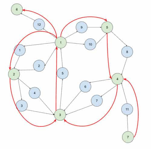
Intuition: After step #3, what we will have is a DAG graph. This is because it assumes that the transactions in a cycle follow the order of time and there will be no backward connection that forms a cycle. Due to the same reason, the transactions that happened earlier will be at the upper level of the DAG graph, and the transactions that happened later will be at the lower level of the DAG graph. Cycle detection cannot be performed yet before performing this step. To detect the cycles, we need to find the upper-level transactions whose sender is the same receiver as its lower-level transaction.

Implementation: Instead of propagating the entire paths, only the ID of each upper-level transaction and its sender ID are pushed down to the lower level. This will make the process very memory efficient and solve challenge #2. Whenever transaction B receives a new transaction ID and sender pair from the upper stream transaction A, it will compare the sender ID from the upper stream with its own receiver account ID. If they are the same, connect a Trans_Trans edge from B to A. Upon the establishment of the connection, the loop will be closed and the lower level transaction B will be flagged as a cycle tail, meaning the last transaction of the cycle.

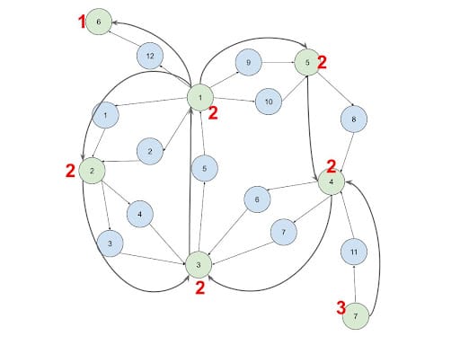
Run SCC on the Transaction Network

Intuition: Once the loops are closed, we have a homogeneous graph with the existence of cycles. We can run an SCC algorithm to detect all the SCC circular patterns that each SCC can contain multiple cycles. Usually, the result of SCC is sufficient to do any downstream analysis. The reasons are:

1. SCC guarantees every pair of transactions to be on at least one cycle
2. Printing all the cycles will result in a very large data size
3. Cycles overlapping with each other are difficult to analyze

Implementation: Simply run SCC on Trans_Trans edges after step #4.

Run Rocha–Thatte on the Transaction Network (Optional)

Intuition: If listing all cycles in the result is absolutely needed, we can still run Rocha–Thatte to calculate the result. However, this time we can use the SCC result as an additional restriction when calculating the cycles. At this point, the Rocha–Thatte calculation will be much more lightweight than directly applying it to the original transactional graph. This is because:

1. No restriction checking is needed when utilizing the Trans_Trans edges created from steps #3 and #4
2. The SCC result from step #5 further filters out unnecessary cycle candidate paths.

Implementation: Simply run Rocha–Thatte on Trans_Trans edges after step #4 while utilizing the SCC result produced in step #5 by filtering out the transactions that are from different SCC.

Experiment

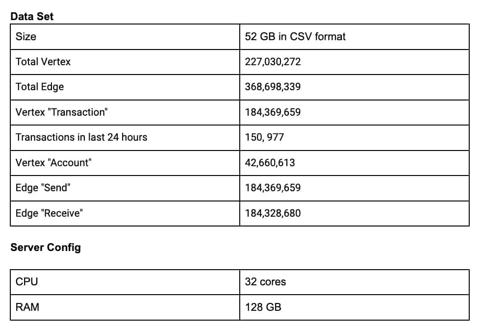
Below are some experiment results proving the effectiveness of the proposed algorithm. We have loaded a 52GB dataset and executed both the plain Rocha–Thatte algorithm and the proposed approach.

The dataset is a public dataset of cryptocurrency history that is between August 2015 and April 2019. The analytics are done on the transactions in the last 24 hours of the dataset.

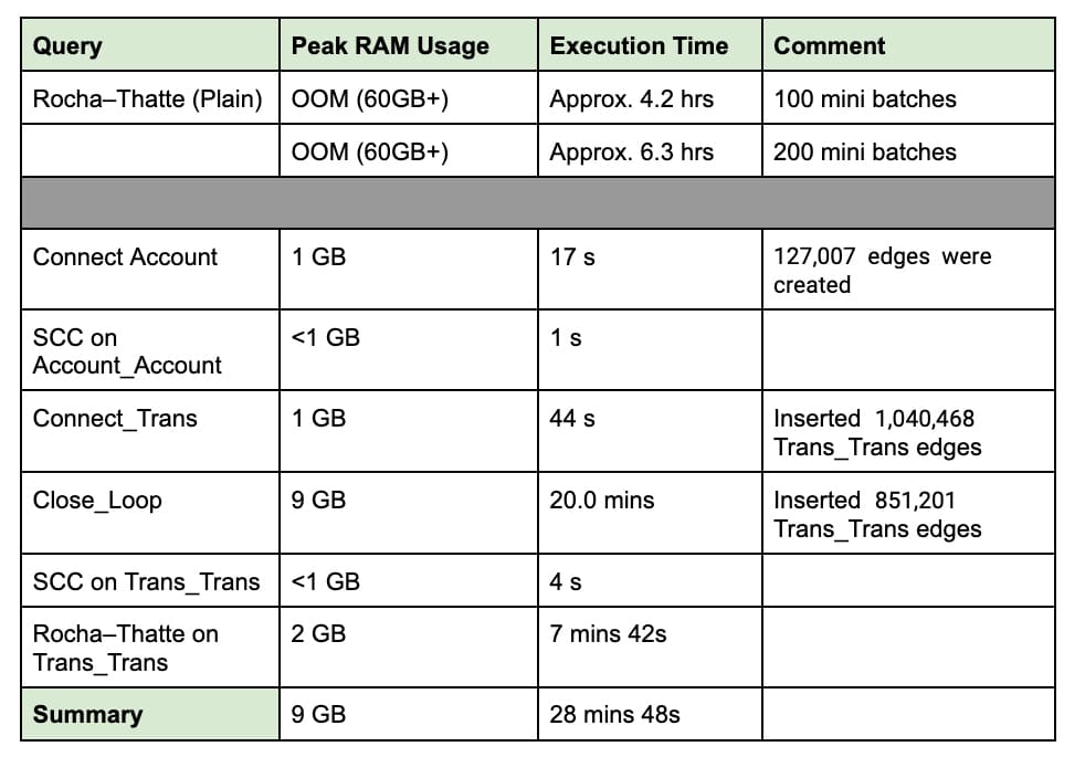
Benchmark

From the benchmark numbers below, we can see that the proposed approach can at least reduce 85% of the memory consumption and uses only about 12.5% of the execution time.

Detect Misbehaving Account Communities

Based on the result of the cycle detection process, additional analysis utilizing the TigerGraph Data Science Library can be performed. We can use the result of cycle detection to identify a complicated community of accounts that conduct circular transactions frequently.

The steps are as follows:

Build Misbehaving Network

When two accounts appeared in the same SCC calculated in step #5, we increment the count of being misbehaving by 1. Then we store the count in an undirected edge between the accounts pairs.

Community Detection

After the complicated network is created, based on the inter-account edges created in the previous step, we can run Louvain, the community detection algorithm. As the result, each community is a group of accounts that frequently perform circular transactions.

Conclusion

With the proposed approach, we can reduce RAM utilization by up to 85% and realize performance up to10x faster than alternative solutions. This makes the cycle detection realistic on large-size transactional data, an important consideration for enterprises working with real-world transaction volumes.