

This article was originally posted on Towards Data Science and is linked to a series, read Part 1 and Part 2. Follow the author, Akash Kaul, on LinkedIn and Medium.
Modeling Publication Data in a Graph
This is part 3 of a series exploring data extraction and modeling. If you’ve followed along with the series so far, welcome back! If you’re new, I’ll give a brief rundown of what we’ve done so far. In Part 1, we explored using NLP and entity extraction on biomedical literature related to Covid-19. In Part 2, we learned how to take our data and model it using TigerGraph Cloud. Check out those articles to get an in-depth look at how we’ve done everything so far.
Now in Part 3, we are going to look at writing graph search queries to easily analyze the data in our graph. You will need a fully formed graph to write queries. You can follow the steps in Part 2 to create a graph from scratch, or you can import the graph we created into TigerGraph Cloud. The graph, along with all of the data we used, can be found here.
To import the graph, create a blank solution following these steps. Once on the homepage of your solution, click Import an Existing Solution.
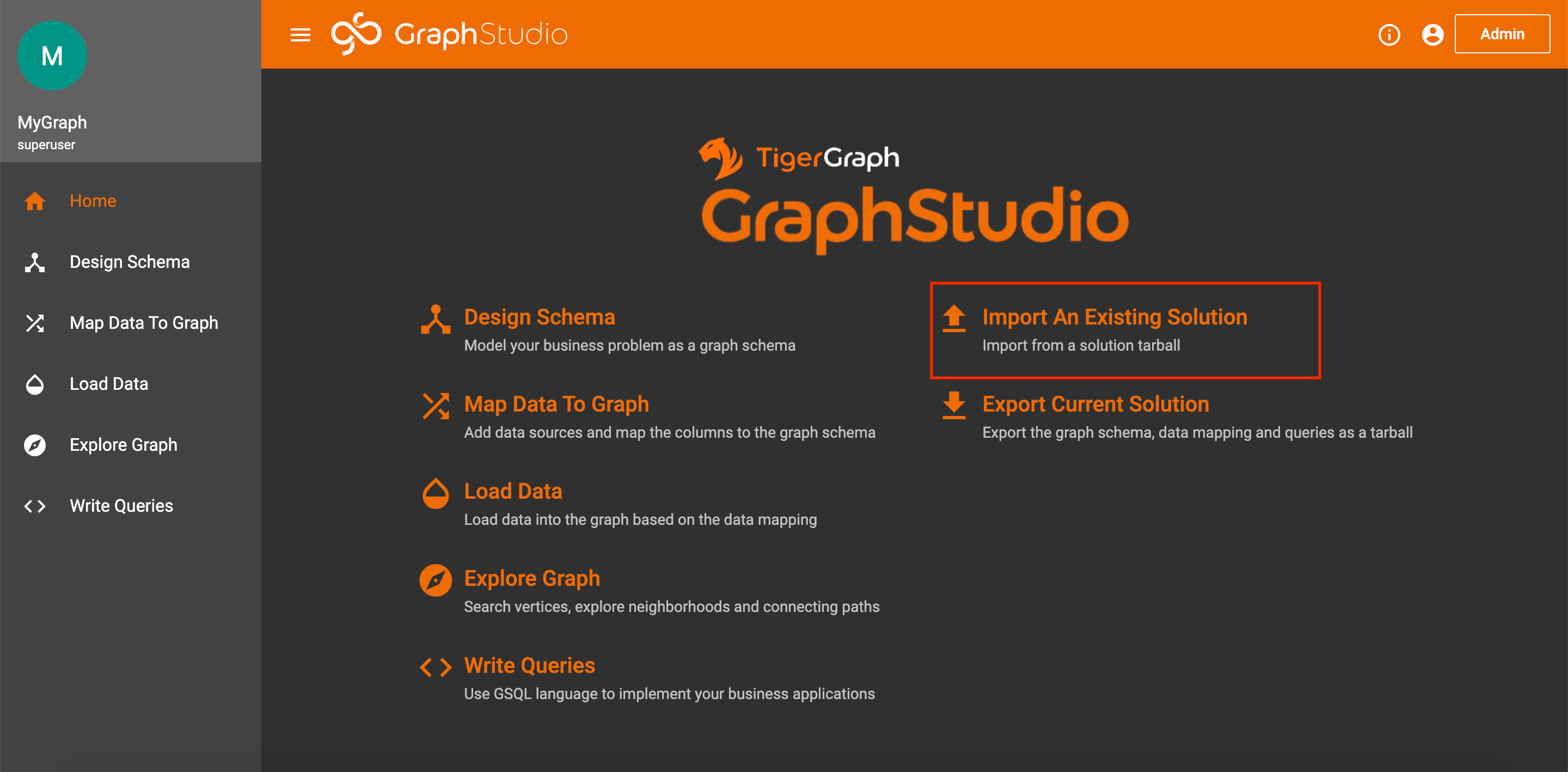
Import Solution on Homepage
Unfortunately, you still have to map and load the data manually. But, I take you through exactly how to do this in Part 2 under agenda items 4 and 5.
What Are Graph Queries?
Before we start writing queries, we should probably understand what they are. Graph queries are essentially commands that search through a graph and perform some operation. Queries can be used to find certain vertices or edges, do computations, or even update the graph. Since graphs also have visual representations, all of this can also be done with a UI, like the one provided by TigerGraph Cloud. But, when working with large amounts of data or when trying to create fine-tuned graph searches, using a visual interface is very inefficient. Hence, we can write queries to quickly traverse a graph and extract or insert whatever data we want.
Query Structure
GSQL offers lots of different methods for querying. We will focus on searches. At the core of graph searches is something called a SELECT statement. As the name suggests, the select statement is used to select a set of vertices or edges. The SELECT statement comes with several parameters to narrow down the focus of your search.
The FROM clause specifies what type of edge or vertex you are choosing.
The WHERE clause lets you declare specific conditions for the vertices or edges.
The ACCUM and POST-ACCUM clauses let you handle Accumulators, which are special GSQL variables that gather information as you search (the information can be numbers, sets of vertices or edges, etc.).
The HAVING clause, similar to the WHERE clause, lets you provide additional conditions; however, these will be applied after the previous clauses.
The ORDER BY clause lets you order the gathered edges or vertices by some attribute value.
Finally, the LIMIT clause constrains the number of results of your search.
You can find all of these details, along with other parameters and query methods, on the TigerGraph documentation page.
Writing Graph Queries
Almost any search you could think of for a graph can be handled with the SELECT statement and its corresponding clauses. To prove that fact, let’s practice writing some queries.
All of the following queries can be found on my GitHub page.
These queries are in order from simplest to most complex.
Publications With a Given License
Goal: Find all publications that fall under a given license type.
Code:
CREATE QUERY LicensePub(String l) FOR GRAPH MyGraph {
/* Finds all publications with a given license type
   Sample Inputs: cc0, cc-by, green-oa, cc-by-nc, no-cc  */
Seed = {LICENSE.*};
Pubs = SELECT p
           FROM Seed:s-(PUB_HAS_LICENSE:e)-PUBLICATION:p
           WHERE s.id == l;
PRINT Pubs[Pubs.id] AS Publications;
}
Explanation: Let’s break down what our code is doing. We want to select all Publication vertices that connect to a specific License vertex. So, we traverse from all LICENSE vertices to all PUBLICATION vertices with the condition that the license id is whatever we specify (i.e. cc0, no-cc, etc.). Then, we just print our results. There are two things to notice in our print statement.
1. If we simply write PRINT Pubs , our output will print the Publications with all of their associated data (title, abstract, etc). So, to filter the output data, we can specify which attributes we want using brackets. In our example, we only print out the ids by writing PRINT Pubs[Pubs.id] .
2. The use of the AS statement is purely cosmetic, and it just changes the name of the resulting list that is printed. This is useful for when you are extracting data to be used in other contexts, but is not necessary for writing queries.
Now, let’s save and install our code. When we run it, we get an input box that looks like this:
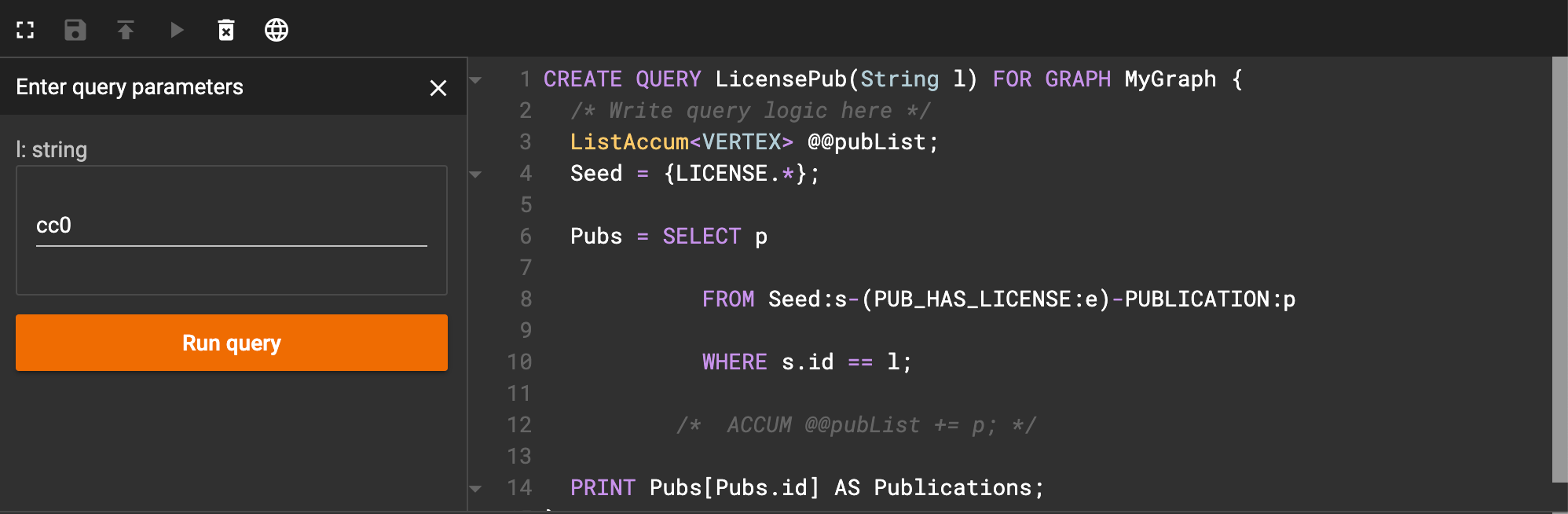
Interface after running license query
As an example, I entered ‘cc0’ as the license code. When I click run query, I get an image that looks like this:
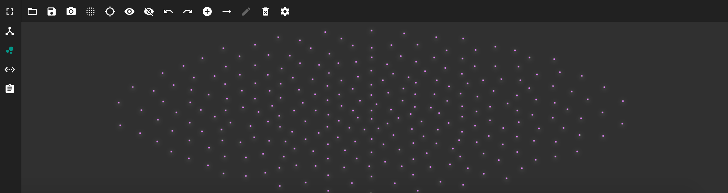
Resulting publication vertices after running license query
This shows each publication vertex that has the license we specified. But, this view is quite messy. We can instead view the JSON output by clicking on the <…> icon on the left side. The JSON output should look like this.
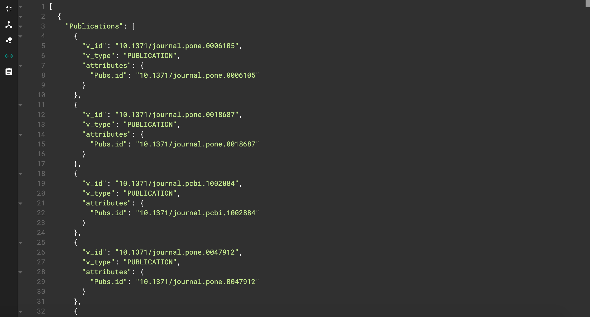
JSON output for license query
This looks much cleaner! We can also see the effects of our print statement adjustments. The name of the resulting list is “Publications”, and the only vertex attribute printed is the id.
For the following queries, I will only show the JSON output.
Author With Most Publications
Goal: Find the author who has written the most publications.
Code:
CREATE QUERY AuthorMostPubs() FOR GRAPH MyGraph {
/* This query finds the author with the most publications
Change the limit to see top 'x' authors */
SumAccum<INT> @pubNum;
Seed={AUTHOR.*};
Author = SELECT a
             FROM Seed:a-()-:t
             ACCUM a.@pubNum +=1
             ORDER BY a.@pubNum DESC
             LIMIT 1;

PRINT Author;
}
Explanation: We start by selecting AUTHOR vertices. Notice that the SELECT statement looks different here. That’s because we didn’t specify the edge or target vertex. Since we know the AUTHOR vertex connects to only the PUBLICATION vertex, we can use this “lazy” syntax to save ourselves from having to specify the edge name and target vertex.
We also get our first look at accumulators (reference the documentation here). In this case, we use a local accumulator called pubNum. A local accumulator acts as a unique variable for each vertex, and a SumAccum is a type of accumulator that stores cumulative sums.
So how does this accumulator work? Well, as we traverse from each AUTHOR vertex to its connected PUBLICATION vertices, we add to our accumulator. So, during the ACCUM clause, the accumulator stores the number of connections (which is also the number of publications) as a variable in each AUTHOR vertex.
The next step uses the ORDER BY clause. We use this to place the resulting authors in descending order of their accumulator value. Thus, the author with the most publications will be at the top of the list
Finally, we use the LIMIT clause to limit the output to 1 author (the first author in the list).
When we run the function, our output looks something like this:
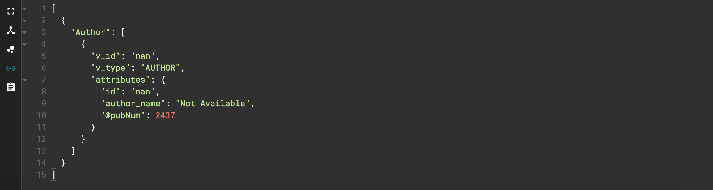
Output for Author query
Notice the author id is “nan”. This is the id used when a publication has no author. So, we can see that 2437 articles have no author listed. This is good information, but not exactly what we’re after. To view more results, change the limit. As an example, I’ll change the limit to 5.
JSON output for author search, limit 5
Now we can see the most-published author has 173 publications (wow that’s a lot!)
Journal With Most Publications
We can run a similar query to the author search but instead search for the journal with the most publications.
Goal: Find the journal(s) with the most publications
Code:
CREATE QUERY JournalMostPubs() FOR GRAPH MyGraph {
/* This query finds the journal with the most publications     Change the limit to find the top 'x' journals  */
SumAccum<INT> @pubNum;
Seed = {PUBLICATION.*};
Pubs = SELECT t
           FROM Seed:s-(PUB_HAS_JOURNAL) -:t

           ACCUM t.@pubNum +=1
           ORDER BY t.@pubNum DESC
           LIMIT 1;
PRINT Pubs[Pubs.id, Pubs.@pubNum] AS Most_Published_Journal;
}
Explanation: The code is essentially the same as before, but we instead search for journals instead of authors. We also use the print filters described earlier to make our output nicer.
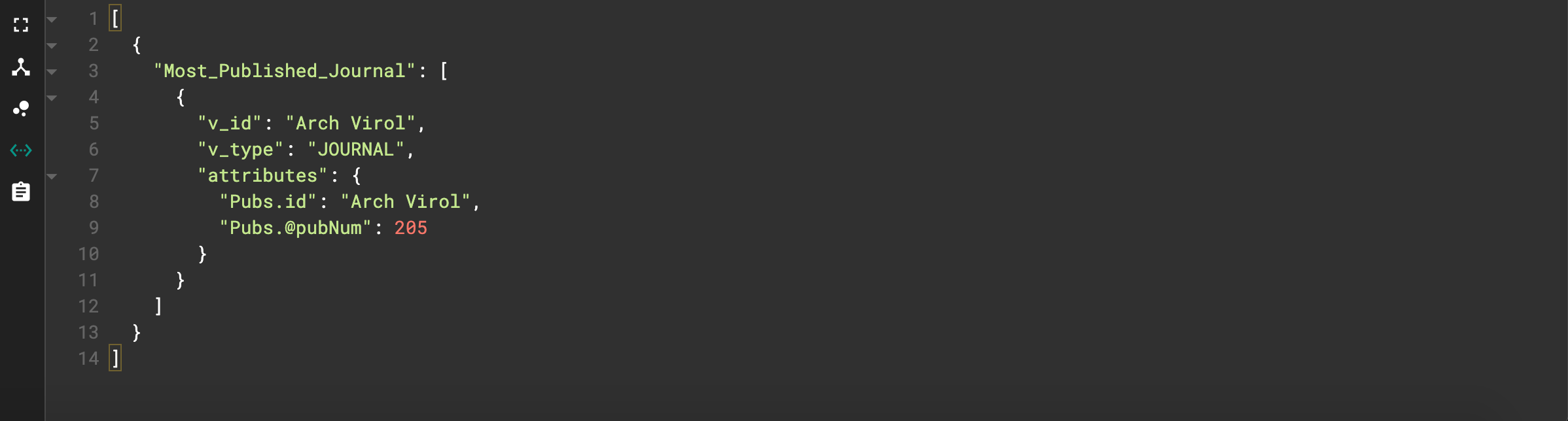
JSON output for journal query
We see that “Arch Virol”, with 205 publications, is the top journal from our search.
Publications with Most References to a Class Type
Goal: Given a class type, find the publications with the most medical terms of that class.
Example class types: DNA, DISEASE, CANCER, ORGANISM, TAXON.
The full list can be found here.
Code:
CREATE QUERY ClassPub(String c, Int k) FOR GRAPH MyGraph{
/* This query finds the top articles related to a class
   Sample Input: CANCER, 5 */
SumAccum<INT> @entNum;
Seed = {CLASS.*};
Ents = SELECT e

          FROM Seed:s-(ENTITY_HAS_CLASS)-ENTITY:e

          WHERE s.id == c;
Pubs = SELECT p
           FROM Ents:e -(PUB_HAS_ENTITY)-PUBLICATION:p

           ACCUM p.@entNum += 1
           ORDER BY p.@entNum DESC
           LIMIT k;
PRINT Pubs[Pubs.id, Pubs.@entNum];
 }
We can now see which publications have the most references to cancer as well as the number of references for each publication.
Similar Publications
Goal: Given a paper, find similar papers based on their shared keywords.
We’ll use Jaccard similarity to determine how closely related 2 papers are. This algorithm essentially computes the number of keywords in common between two papers over the total number of keywords. You can read more about the algorithm here. You can see an example of this formula in action, as well as many other cool graph formulas, on the TigerGraph GitHub.
CREATE QUERY SimilarEnt(STRING doi, INT top) FOR GRAPH MyGraph {
/* Use Jaccard Similarity to find top similar articles of a given article based on the key medical terms used
Sample Input: 10.1186/1471-2164-7-117, 5 */
SumAccum<INT> @intersection_size, @@set_sizeA, @set_sizeB;
SumAccum<FLOAT> @similarity;
VERTEX check;
Seed = {PUBLICATION.*};
Start = SELECT p
            FROM Seed:p
            WHERE p.id == doi
            ACCUM check = p,
                         @@set_sizeA+=p.outdegree("PUB_HAS_ENTITY");
Subjects = SELECT t
            FROM Start:s-(PUB_HAS_ENTITY)-:t;
Others = SELECT t
            FROM Subjects:s -(PUB_HAS_ENTITY) - :t
            WHERE t!= check
            ACCUM t.@intersection_size +=1,
                  t.@set_sizeB = t.outdegree("PUB_HAS_ENTITY")

            POST-ACCUM t.@similarity = t.@intersection_size
                       *1.0/(@@set_sizeA+t.@set_sizeB-
                       t.@intersection_size)
            ORDER BY t.@similarity DESC
            LIMIT top;
PRINT Start[Start.id] AS SOURCE_PUBLICATION;
PRINT Others[Others.@similarity] AS SIMILAR_PUBLICATIONS;
Explanation: We start by creating 4 accumulators. Each one represents a value used in the Jaccard formula. For our first SELECT statement, we select the publication matching the input doi and collect all of the edges connected to that vertex into an accumulator. For our second statement, we select all of the entities in that publication. For our third statement, we find all of the publications with any number of the entities we just gathered and find the intersection size (the number of entities in common with the original paper). Finally, we calculate our Jaccard index and sort publications with the highest similarities to be at the top of our output list.
Let’s see an example. I used doi=10.1186/s40413–016–0096–1 and top=5.
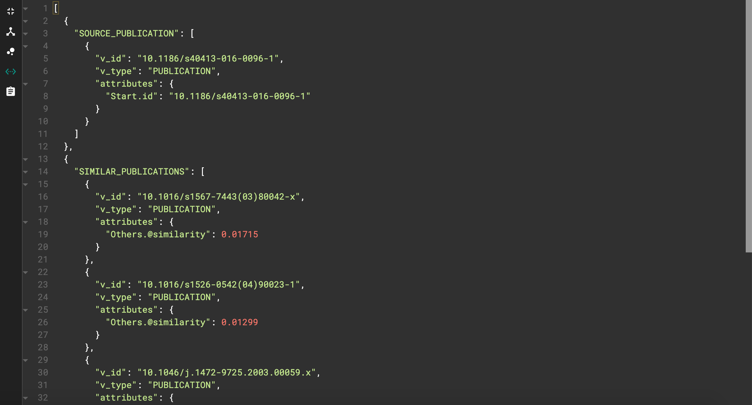
JSON output for similarity query
We can see our starting publication as well as the top 5 similar publications, each with their respective similarity score.
Conclusion
If you followed along with this article, I applaud you! This material is not easy, and learning a new language like GSQL can be tricky. I hope you found this walkthrough of GSQL queries insightful. I highly recommend reading my other papers to get a better background for everything we’ve covered today. If you’re looking to check out more query algorithms and structures, check out the TigerGraph documentation for GSQL. If you’re looking for more content, stay tuned! I’ll be releasing Part 4 shortly. In this final part of the series, I’ll cover how to use our graph database and queries to output information that we can visually represent using the UI platform Dash from Plotly. With that, if you have followed along for all 4 parts, you will finish a full, end-to-end application!
If you enjoyed this paper, be sure to check out my other papers and follow me for more content like this!
Resources
- https://towardsdatascience.com/using-scispacy-for-named-entity-recognition-785389e7918d
- https://towardsdatascience.com/linking-documents-in-a-semantic-graph-732ab511a01e
- https://gofile.io/d/fyijVS
- https://www.youtube.com/watch?v=JARd9ULRP_I
- https://docs.tigergraph.com/dev/gsql-ref/querying/accumulators
- https://docs.tigergraph.com/dev/gsql-ref/querying/select-statement#select-statement-data-flow
- https://github.com/akash-kaul/GSQL-Query-Searches.git
- https://allenai.github.io/scispacy/
- https://github.com/tigergraph/gsql-graph-algorithms/blob/master/algorithms/schema-free/jaccard_nbor_ap_json.gsql
- https://docs.tigergraph.com/
- https://plotly.com/dash/